How many ways are supported to visualise gene-active networks?
Notes:
# The dnet package supports two ways to visualise the identified networks/graphs: 1) the network itself as a single display, 2) the same network but with multiple colorings/displays according to samples.
# To demonstrate the visuals supported, we use a random graph generated according to the ER model, and only keep the largest component.
g <- erdos.renyi.game(100, 1/100)
g <- dNetInduce(g, nodes_query=V(g))
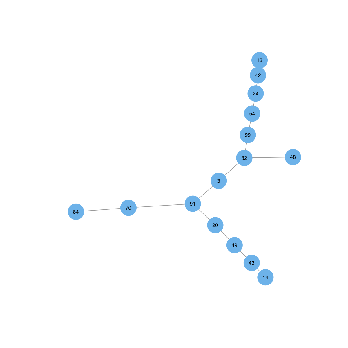
# To display the network itself, the key setting is the layout. Since the network is represented as an object of class 'igraph', the layouts supported in the 'igraph' package can be found in the layout page. Below is an example using a force-based algorithm proposed by Fruchterman and Reingold:
visNet(g, layout=layout.fruchterman.reingold)
# Additionally, the dnet package also uses two other layouts/diagrams: 1) arc diagram in one-dimensional layout, and 2) circle diagram.
# To better display the network, it is advisable to incorporate community information. In doing so, we first identify communities based on a spin-glass model and simulated annealing.
com <- igraph::spinglass.community(g, spins=25)
 vgroups <- com$membership
## color nodes: according to communities
mcolors <- visColormap(colormap="rainbow")(length(com))
vcolors <- mcolors[vgroups]
## size nodes: according to degrees
vdegrees <- igraph::degree(g)
## sort nodes: first by communities and then degrees
df <- data.frame(ind=1:vcount(g), vgroups, vdegrees)
ordering <- df[order(vgroups,vdegrees),]$ind
# Now, make comparsions between different layouts
## using 1-dimensional arc diagram
visNetArc(g, ordering=ordering, vertex.label.color=vcolors, vertex.color=vcolors, vertex.frame.color=vcolors, vertex.size=log(vdegrees)+0.1)
## using circle diagram (drawn into a single circle)
visNetCircle(g, colormap="rainbow", com=com, ordering=ordering)
## using circle diagram (drawn into multlpe circles: one circle per community)
visNetCircle(g, colormap="rainbow", com=com, circles="multiple", ordering=ordering)
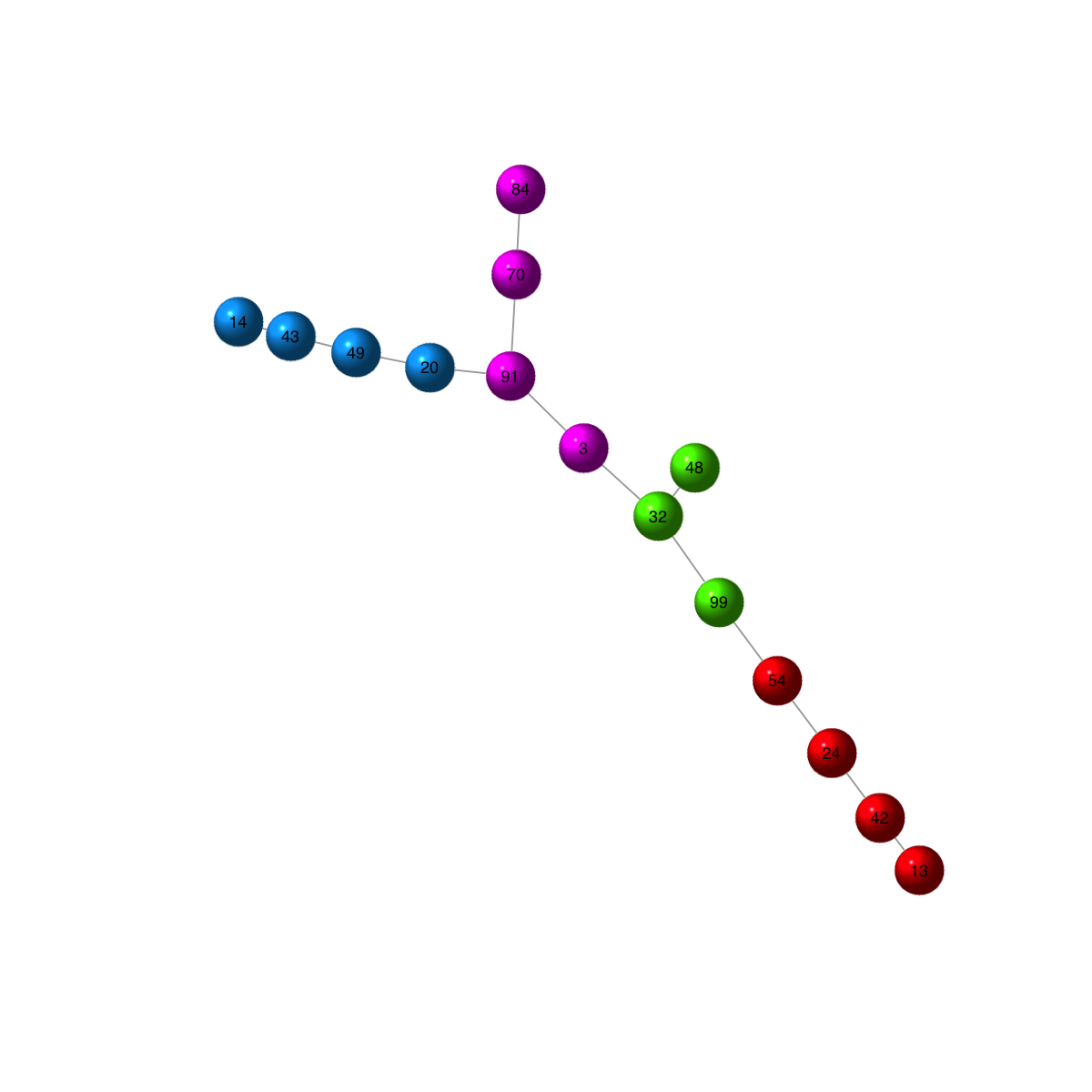
## using a force-based algorithm proposed by Fruchterman and Reingold
visNet(g, colormap="rainbow", layout=layout.fruchterman.reingold, vertex.color=vcolors, vertex.frame.color=vcolors, vertex.shape="sphere")
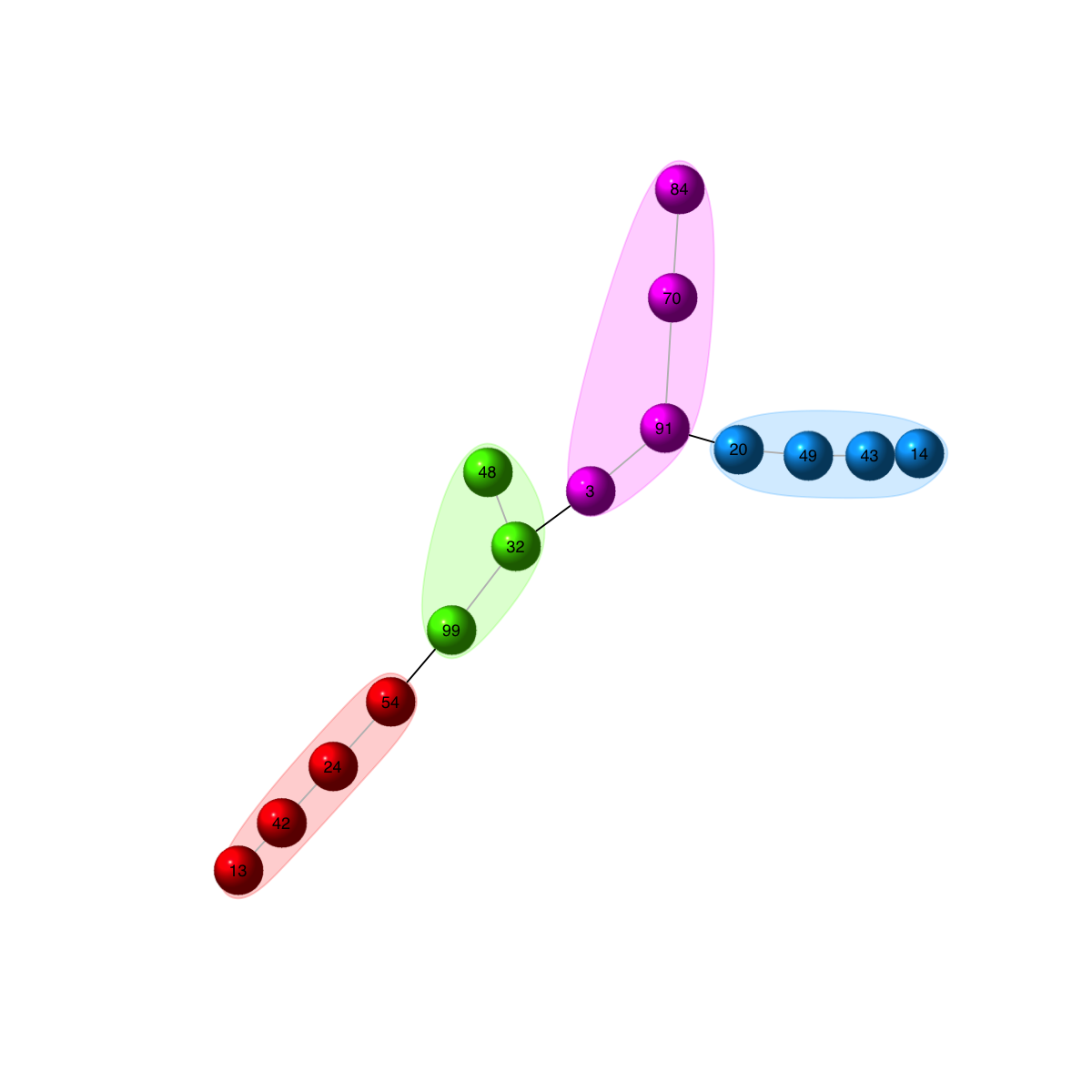
## when using force-based layout, it is also useful to highlight the communities in the background, and have edges being colored differently according whether an edge lies within a community or between communities.
mark.groups <- igraph::communities(com)
vgroups <- com$membership
## color nodes: according to communities
mcolors <- visColormap(colormap="rainbow")(length(com))
vcolors <- mcolors[vgroups]
## size nodes: according to degrees
vdegrees <- igraph::degree(g)
## sort nodes: first by communities and then degrees
df <- data.frame(ind=1:vcount(g), vgroups, vdegrees)
ordering <- df[order(vgroups,vdegrees),]$ind
# Now, make comparsions between different layouts
## using 1-dimensional arc diagram
visNetArc(g, ordering=ordering, vertex.label.color=vcolors, vertex.color=vcolors, vertex.frame.color=vcolors, vertex.size=log(vdegrees)+0.1)
## using circle diagram (drawn into a single circle)
visNetCircle(g, colormap="rainbow", com=com, ordering=ordering)
## using circle diagram (drawn into multlpe circles: one circle per community)
visNetCircle(g, colormap="rainbow", com=com, circles="multiple", ordering=ordering)
## using a force-based algorithm proposed by Fruchterman and Reingold
visNet(g, colormap="rainbow", layout=layout.fruchterman.reingold, vertex.color=vcolors, vertex.frame.color=vcolors, vertex.shape="sphere")
## when using force-based layout, it is also useful to highlight the communities in the background, and have edges being colored differently according whether an edge lies within a community or between communities.
mark.groups <- igraph::communities(com)
 mark.col <- visColoralpha(mcolors, alpha=0.2)
mark.border <- visColoralpha(mcolors, alpha=0.2)
edge.color <- c("grey", "black")[igraph::crossing(com,g)+1]
visNet(g, colormap="rainbow", glayout=layout.fruchterman.reingold, vertex.color=vcolors, vertex.frame.color=vcolors, vertex.shape="sphere", mark.groups=mark.groups, mark.col=mark.col, mark.border=mark.border, mark.shape=1, mark.expand=10, edge.color=edge.color)
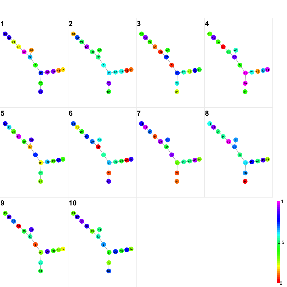
# Now, let us look at visualising the same network but with the multiple colorings/displays according to samples.
# Assume we have 10 samples, each containing numeric information about nodes in the graph:
nnodes <- vcount(g)
mark.col <- visColoralpha(mcolors, alpha=0.2)
mark.border <- visColoralpha(mcolors, alpha=0.2)
edge.color <- c("grey", "black")[igraph::crossing(com,g)+1]
visNet(g, colormap="rainbow", glayout=layout.fruchterman.reingold, vertex.color=vcolors, vertex.frame.color=vcolors, vertex.shape="sphere", mark.groups=mark.groups, mark.col=mark.col, mark.border=mark.border, mark.shape=1, mark.expand=10, edge.color=edge.color)
# Now, let us look at visualising the same network but with the multiple colorings/displays according to samples.
# Assume we have 10 samples, each containing numeric information about nodes in the graph:
nnodes <- vcount(g)
 nsamples <- 10
data <- matrix(runif(nnodes*nsamples), nrow=nnodes, ncol=nsamples)
rownames(data) <- V(g)$name
# In the dnet package, these sample-specific network visuals can be simply as they are provided, or samples being self-organised onto 2D landscape.
## simply as they are provided
visNetMul(g, colormap="rainbow", data=data, glayout=layout.fruchterman.reingold)
## being self-organised onto 2D sample landscape (ie a sheet-shape rectangle grid)
sReorder <- dNetReorder(g, data, feature="node", node.normalise="none")
Start at 2017-03-27 20:08:19
First, define topology of a map grid (2017-03-27 20:08:19)...
Second, initialise the codebook matrix (36 X 15) using 'linear' initialisation, given a topology and input data (2017-03-27 20:08:19)...
Third, get training at the rough stage (2017-03-27 20:08:19)...
1 out of 360 (2017-03-27 20:08:19)
36 out of 360 (2017-03-27 20:08:19)
72 out of 360 (2017-03-27 20:08:19)
108 out of 360 (2017-03-27 20:08:19)
144 out of 360 (2017-03-27 20:08:19)
180 out of 360 (2017-03-27 20:08:19)
216 out of 360 (2017-03-27 20:08:19)
252 out of 360 (2017-03-27 20:08:19)
288 out of 360 (2017-03-27 20:08:19)
324 out of 360 (2017-03-27 20:08:19)
360 out of 360 (2017-03-27 20:08:19)
Fourth, get training at the finetune stage (2017-03-27 20:08:19)...
1 out of 1440 (2017-03-27 20:08:19)
144 out of 1440 (2017-03-27 20:08:19)
288 out of 1440 (2017-03-27 20:08:19)
432 out of 1440 (2017-03-27 20:08:19)
576 out of 1440 (2017-03-27 20:08:19)
720 out of 1440 (2017-03-27 20:08:19)
864 out of 1440 (2017-03-27 20:08:20)
1008 out of 1440 (2017-03-27 20:08:20)
1152 out of 1440 (2017-03-27 20:08:20)
1296 out of 1440 (2017-03-27 20:08:20)
1440 out of 1440 (2017-03-27 20:08:20)
Next, identify the best-matching hexagon/rectangle for the input data (2017-03-27 20:08:20)...
Finally, append the response data (hits and mqe) into the sMap object (2017-03-27 20:08:20)...
Below are the summaries of the training results:
dimension of input data: 10x15
xy-dimension of map grid: xdim=6, ydim=6, r=3
grid lattice: rect
grid shape: sheet
dimension of grid coord: 36x2
initialisation method: linear
dimension of codebook matrix: 36x15
mean quantization error: 0.295066255049138
Below are the details of trainology:
training algorithm: sequential
alpha type: invert
training neighborhood kernel: gaussian
trainlength (x input data length): 36 at rough stage; 144 at finetune stage
radius (at rough stage): from 1 to 1
radius (at finetune stage): from 1 to 1
End at 2017-03-27 20:08:20
Runtime in total is: 1 secs
nsamples <- 10
data <- matrix(runif(nnodes*nsamples), nrow=nnodes, ncol=nsamples)
rownames(data) <- V(g)$name
# In the dnet package, these sample-specific network visuals can be simply as they are provided, or samples being self-organised onto 2D landscape.
## simply as they are provided
visNetMul(g, colormap="rainbow", data=data, glayout=layout.fruchterman.reingold)
## being self-organised onto 2D sample landscape (ie a sheet-shape rectangle grid)
sReorder <- dNetReorder(g, data, feature="node", node.normalise="none")
Start at 2017-03-27 20:08:19
First, define topology of a map grid (2017-03-27 20:08:19)...
Second, initialise the codebook matrix (36 X 15) using 'linear' initialisation, given a topology and input data (2017-03-27 20:08:19)...
Third, get training at the rough stage (2017-03-27 20:08:19)...
1 out of 360 (2017-03-27 20:08:19)
36 out of 360 (2017-03-27 20:08:19)
72 out of 360 (2017-03-27 20:08:19)
108 out of 360 (2017-03-27 20:08:19)
144 out of 360 (2017-03-27 20:08:19)
180 out of 360 (2017-03-27 20:08:19)
216 out of 360 (2017-03-27 20:08:19)
252 out of 360 (2017-03-27 20:08:19)
288 out of 360 (2017-03-27 20:08:19)
324 out of 360 (2017-03-27 20:08:19)
360 out of 360 (2017-03-27 20:08:19)
Fourth, get training at the finetune stage (2017-03-27 20:08:19)...
1 out of 1440 (2017-03-27 20:08:19)
144 out of 1440 (2017-03-27 20:08:19)
288 out of 1440 (2017-03-27 20:08:19)
432 out of 1440 (2017-03-27 20:08:19)
576 out of 1440 (2017-03-27 20:08:19)
720 out of 1440 (2017-03-27 20:08:19)
864 out of 1440 (2017-03-27 20:08:20)
1008 out of 1440 (2017-03-27 20:08:20)
1152 out of 1440 (2017-03-27 20:08:20)
1296 out of 1440 (2017-03-27 20:08:20)
1440 out of 1440 (2017-03-27 20:08:20)
Next, identify the best-matching hexagon/rectangle for the input data (2017-03-27 20:08:20)...
Finally, append the response data (hits and mqe) into the sMap object (2017-03-27 20:08:20)...
Below are the summaries of the training results:
dimension of input data: 10x15
xy-dimension of map grid: xdim=6, ydim=6, r=3
grid lattice: rect
grid shape: sheet
dimension of grid coord: 36x2
initialisation method: linear
dimension of codebook matrix: 36x15
mean quantization error: 0.295066255049138
Below are the details of trainology:
training algorithm: sequential
alpha type: invert
training neighborhood kernel: gaussian
trainlength (x input data length): 36 at rough stage; 144 at finetune stage
radius (at rough stage): from 1 to 1
radius (at finetune stage): from 1 to 1
End at 2017-03-27 20:08:20
Runtime in total is: 1 secs
 visNetReorder(g, colormap="rainbow", data=data, sReorder)
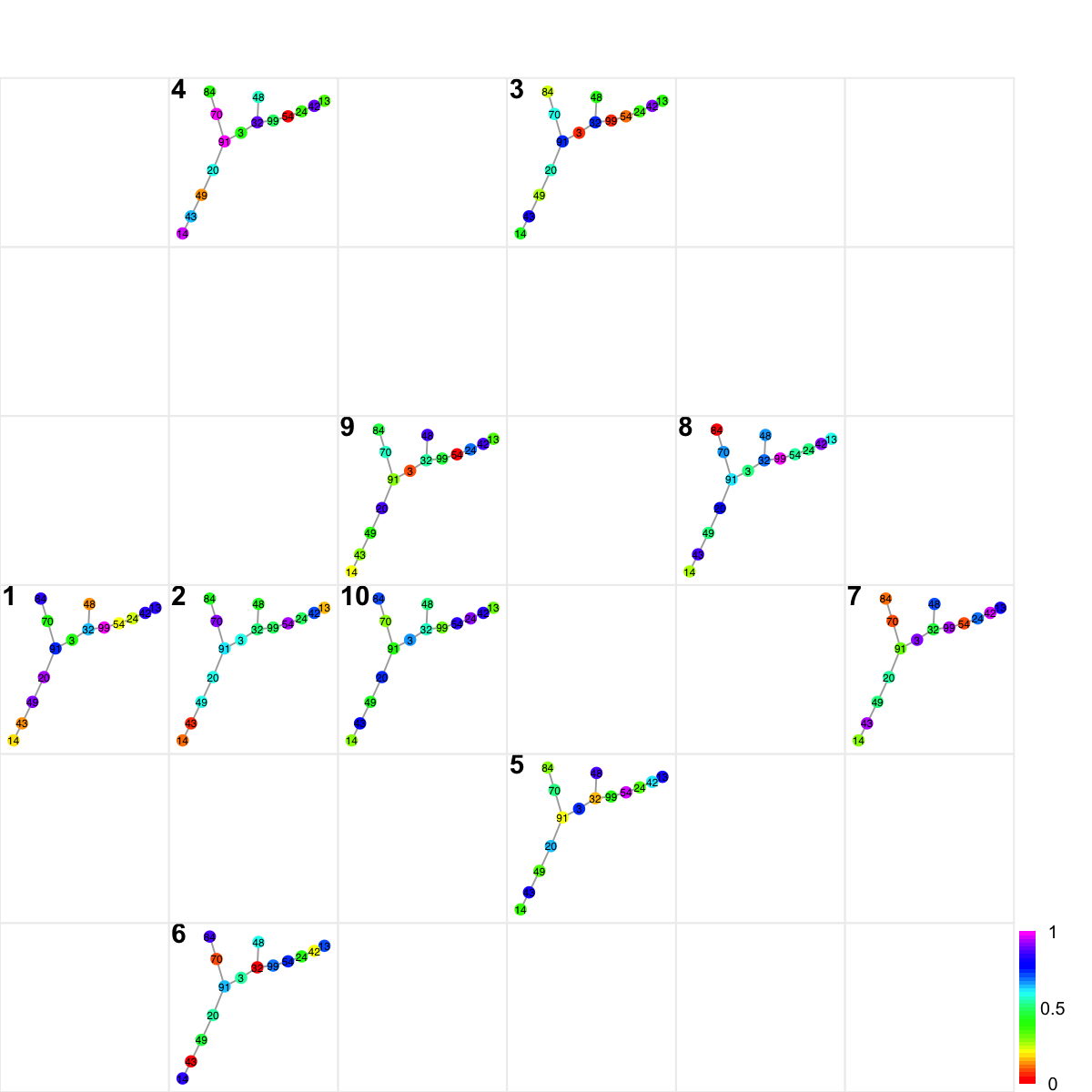
## By default, 2D sample landscape is built based on node features without considering node degrees. To take into account the connectivity in the network, the information used can be on edges which are transformed from information on nodes: input data and degree. In doing so, the transformed matrix of network edges × samples are used for self-organising samples onto 2D landscape (implemented in the 'supraHex' package).
sReorder <- dNetReorder(g, data, feature="edge", node.normalise="degree")
Start at 2017-03-27 20:08:22
First, define topology of a map grid (2017-03-27 20:08:22)...
Second, initialise the codebook matrix (36 X 14) using 'linear' initialisation, given a topology and input data (2017-03-27 20:08:22)...
Third, get training at the rough stage (2017-03-27 20:08:22)...
1 out of 360 (2017-03-27 20:08:22)
36 out of 360 (2017-03-27 20:08:22)
72 out of 360 (2017-03-27 20:08:22)
108 out of 360 (2017-03-27 20:08:22)
144 out of 360 (2017-03-27 20:08:22)
180 out of 360 (2017-03-27 20:08:22)
216 out of 360 (2017-03-27 20:08:22)
252 out of 360 (2017-03-27 20:08:22)
288 out of 360 (2017-03-27 20:08:22)
324 out of 360 (2017-03-27 20:08:22)
360 out of 360 (2017-03-27 20:08:22)
Fourth, get training at the finetune stage (2017-03-27 20:08:22)...
1 out of 1440 (2017-03-27 20:08:22)
144 out of 1440 (2017-03-27 20:08:22)
288 out of 1440 (2017-03-27 20:08:22)
432 out of 1440 (2017-03-27 20:08:22)
576 out of 1440 (2017-03-27 20:08:22)
720 out of 1440 (2017-03-27 20:08:22)
864 out of 1440 (2017-03-27 20:08:22)
1008 out of 1440 (2017-03-27 20:08:22)
1152 out of 1440 (2017-03-27 20:08:22)
1296 out of 1440 (2017-03-27 20:08:22)
1440 out of 1440 (2017-03-27 20:08:22)
Next, identify the best-matching hexagon/rectangle for the input data (2017-03-27 20:08:22)...
Finally, append the response data (hits and mqe) into the sMap object (2017-03-27 20:08:22)...
Below are the summaries of the training results:
dimension of input data: 10x14
xy-dimension of map grid: xdim=6, ydim=6, r=3
grid lattice: rect
grid shape: sheet
dimension of grid coord: 36x2
initialisation method: linear
dimension of codebook matrix: 36x14
mean quantization error: 0.082028513549375
Below are the details of trainology:
training algorithm: sequential
alpha type: invert
training neighborhood kernel: gaussian
trainlength (x input data length): 36 at rough stage; 144 at finetune stage
radius (at rough stage): from 1 to 1
radius (at finetune stage): from 1 to 1
End at 2017-03-27 20:08:22
Runtime in total is: 0 secs
visNetReorder(g, colormap="rainbow", data=data, sReorder)
## By default, 2D sample landscape is built based on node features without considering node degrees. To take into account the connectivity in the network, the information used can be on edges which are transformed from information on nodes: input data and degree. In doing so, the transformed matrix of network edges × samples are used for self-organising samples onto 2D landscape (implemented in the 'supraHex' package).
sReorder <- dNetReorder(g, data, feature="edge", node.normalise="degree")
Start at 2017-03-27 20:08:22
First, define topology of a map grid (2017-03-27 20:08:22)...
Second, initialise the codebook matrix (36 X 14) using 'linear' initialisation, given a topology and input data (2017-03-27 20:08:22)...
Third, get training at the rough stage (2017-03-27 20:08:22)...
1 out of 360 (2017-03-27 20:08:22)
36 out of 360 (2017-03-27 20:08:22)
72 out of 360 (2017-03-27 20:08:22)
108 out of 360 (2017-03-27 20:08:22)
144 out of 360 (2017-03-27 20:08:22)
180 out of 360 (2017-03-27 20:08:22)
216 out of 360 (2017-03-27 20:08:22)
252 out of 360 (2017-03-27 20:08:22)
288 out of 360 (2017-03-27 20:08:22)
324 out of 360 (2017-03-27 20:08:22)
360 out of 360 (2017-03-27 20:08:22)
Fourth, get training at the finetune stage (2017-03-27 20:08:22)...
1 out of 1440 (2017-03-27 20:08:22)
144 out of 1440 (2017-03-27 20:08:22)
288 out of 1440 (2017-03-27 20:08:22)
432 out of 1440 (2017-03-27 20:08:22)
576 out of 1440 (2017-03-27 20:08:22)
720 out of 1440 (2017-03-27 20:08:22)
864 out of 1440 (2017-03-27 20:08:22)
1008 out of 1440 (2017-03-27 20:08:22)
1152 out of 1440 (2017-03-27 20:08:22)
1296 out of 1440 (2017-03-27 20:08:22)
1440 out of 1440 (2017-03-27 20:08:22)
Next, identify the best-matching hexagon/rectangle for the input data (2017-03-27 20:08:22)...
Finally, append the response data (hits and mqe) into the sMap object (2017-03-27 20:08:22)...
Below are the summaries of the training results:
dimension of input data: 10x14
xy-dimension of map grid: xdim=6, ydim=6, r=3
grid lattice: rect
grid shape: sheet
dimension of grid coord: 36x2
initialisation method: linear
dimension of codebook matrix: 36x14
mean quantization error: 0.082028513549375
Below are the details of trainology:
training algorithm: sequential
alpha type: invert
training neighborhood kernel: gaussian
trainlength (x input data length): 36 at rough stage; 144 at finetune stage
radius (at rough stage): from 1 to 1
radius (at finetune stage): from 1 to 1
End at 2017-03-27 20:08:22
Runtime in total is: 0 secs
 visNetReorder(g, colormap="rainbow", data=data, sReorder)
)
)
)
)
)