# This is a demo for human embryo dataset from Fang et al
#
# This human embryo expression dataset (available from
http://www.ncbi.nlm.nih.gov/pubmed/20643359) involves six successive developmental stages (S9-S14) with three replicates (R1-R3) for each stage, including:
## Fang: an expression matrix of 5,441 genes X 18 samples;
## Fang.geneinfo: a matrix of 5,441 X 3 containing gene information;
## Fang.sampleinfo: a matrix of 18 X 3 containing sample information.
###############################################################################
library(dnet)
# Load or install packages specifically used in this demo
for(pkg in c("Biobase","limma")){
if(!require(pkg, character.only=T)){
source("http://bioconductor.org/biocLite.R")
biocLite(pkg)
lapply(pkg, library, character.only=T)
}
}
# import data containing three variables ('Fang', 'Fang.geneinfo' and 'Fang.sampleinfo')
data(Fang)
data <- Fang
fdata <- as.data.frame(Fang.geneinfo[,2:3])
rownames(fdata) <- Fang.geneinfo[,1]
pdata <- as.data.frame(Fang.sampleinfo[,2:3])
rownames(pdata) <- Fang.sampleinfo[,1]
# create the 'eset' object
colmatch <- match(rownames(pdata),colnames(data))
rowmatch <- match(rownames(fdata),rownames(data))
data <- data[rowmatch,colmatch]
eset <- new("ExpressionSet", exprs=as.matrix(data), phenoData=as(pdata,"AnnotatedDataFrame"), featureData=as(fdata,"AnnotatedDataFrame"))
# A function to convert probeset-centric to entrezgene-centric expression levels
prob2gene <- function(eset){
fdat <- fData(eset)
tmp <- as.matrix(unique(fdat[c("EntrezGene", "Symbol")]))
forder <- tmp[order(as.numeric(tmp[,1])),]
forder <- forder[!is.na(forder[,1]),]
rownames(forder) <- forder[,2]
system.time({
dat <- exprs(eset)
edat <- matrix(data=NA, nrow=nrow(forder), ncol=ncol(dat))
for (i in 1:nrow(forder)){
ind <- which(fdat$EntrezGene==as.numeric(forder[i,1]))
if (length(ind) == 1){
edat[i,] <- dat[ind,]
}else{
edat[i,] <- apply(dat[ind,],2,mean)
}
}
})
rownames(edat) <- rownames(forder) # as gene symbols
colnames(edat) <- rownames(pData(eset))
esetGene <- new('ExpressionSet',exprs=data.frame(edat),phenoData=as(pData(eset),"AnnotatedDataFrame"),featureData=as(data.frame(forder),"AnnotatedDataFrame"))
return(esetGene)
}
esetGene <- prob2gene(eset)
esetGene
ExpressionSet (storageMode: lockedEnvironment)
assayData: 4139 features, 18 samples
element names: exprs
protocolData: none
phenoData
sampleNames: S9_R1 S9_R2 ... S14_R3 (18 total)
varLabels: Stage Replicate
varMetadata: labelDescription
featureData
featureNames: A2M AADAC ... LOC100131613 (4139 total)
fvarLabels: EntrezGene Symbol
fvarMetadata: labelDescription
experimentData: use 'experimentData(object)'
Annotation:
'org.Hs.string' (from http://supfam.org/dnet/RData/1.0.7/org.Hs.string.RData) has been loaded into the working environment
org.Hs.string
IGRAPH UN-- 18492 728141 --
+ attr: name (v/c), seqid (v/c), geneid (v/n), symbol (v/c),
| description (v/c), neighborhood_score (e/n), fusion_score (e/n),
| cooccurence_score (e/n), coexpression_score (e/n), experimental_score
| (e/n), database_score (e/n), textmining_score (e/n), combined_score
| (e/n)
+ edges (vertex names):
[1] 3025671--3031737 3021358--3027795 3021358--3027929 3021358--3027741
[5] 3024278--3029186 3029373--3031543 3031543--3034385 3019006--3030823
[9] 3015391--3030823 3021191--3028634 3021191--3024550 3021191--3033402
[13] 3031876--3031959 3015324--3031959 3023108--3033954 3016546--3020273
+ ... omitted several edges
# extract network that only contains genes in esetGene
ind <- match(V(org.Hs.string)$symbol, rownames(esetGene))
## for extracted expression
esetGeneSub <- esetGene[ind[!is.na(ind)],]
esetGeneSub
ExpressionSet (storageMode: lockedEnvironment)
assayData: 3734 features, 18 samples
element names: exprs
protocolData: none
phenoData
sampleNames: S9_R1 S9_R2 ... S14_R3 (18 total)
varLabels: Stage Replicate
varMetadata: labelDescription
featureData
featureNames: PPP1R12B KLF10 ... SOX13 (3734 total)
fvarLabels: EntrezGene Symbol
fvarMetadata: labelDescription
experimentData: use 'experimentData(object)'
Annotation:
IGRAPH UN-- 3623 63805 --
+ attr: name (v/c), seqid (v/c), geneid (v/n), symbol (v/c),
| description (v/c)
+ edges (vertex names):
[1] PPP1R12B--NUAK1 PPP1R12B--MYLPF PPP1R12B--MAP2 PPP1R12B--ROCK1
[5] PPP1R12B--RPSA PPP1R12B--DIAPH2 PPP1R12B--PDLIM7 PPP1R12B--PPP1CC
[9] PPP1R12B--MYH3 PPP1R12B--PDLIM5 PPP1R12B--ACTN2 PPP1R12B--LDB3
[13] PPP1R12B--HSPA8 PPP1R12B--MYL2 PPP1R12B--FRMD4A PPP1R12B--MYH7
[17] PPP1R12B--MYL6 PPP1R12B--MYO10 PPP1R12B--PCBP2 PPP1R12B--MAPT
[21] PPP1R12B--ACTN1 PPP1R12B--T PPP1R12B--EZR PPP1R12B--MSN
[25] PPP1R12B--CDC42BPA PPP1R12B--MYH6 PPP1R12B--MYL9 PPP1R12B--NUAK2
+ ... omitted several edges
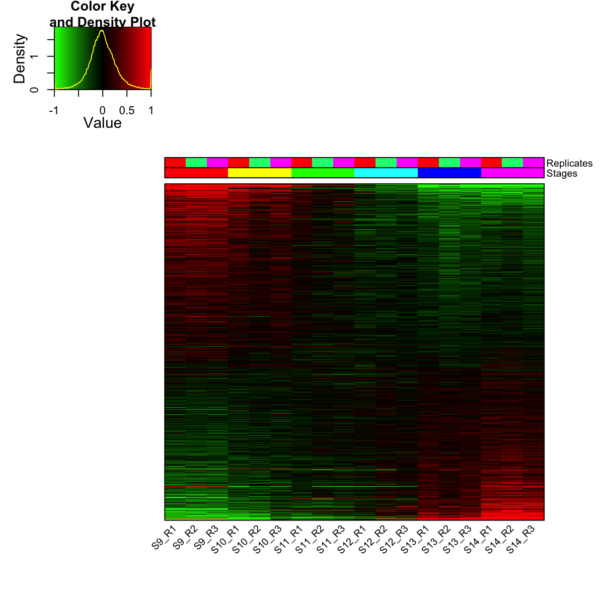
# prepare the expression matrix
D <- as.matrix(exprs(esetGene))
D <- D - as.matrix(apply(D,1,mean),ncol=1)[,rep(1,ncol(D))]
# heatmap of expression matrix with rows ordered according the dominant patterns
sorted <- sort.int(D %*% svd(D)$v[,1], decreasing=T, index.return=T)
mat_data <- D[sorted$ix,]
# prepare colors for the column sidebar
# color for stages (S9-S14)
stages <- sub("_.*","",colnames(mat_data))
sta_lvs <- unique(stages)
sta_color <- visColormap(colormap="rainbow")(length(sta_lvs))
col_stages <- sapply(stages, function(x) sta_color[x==sta_lvs])
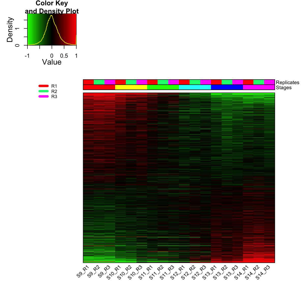
# color for replicates (R1-R3)
replicates <- sub(".*_","",colnames(mat_data))
rep_lvs <- unique(replicates)
rep_color <- visColormap(colormap="rainbow")(length(rep_lvs))
col_replicates <- sapply(replicates, function(x) rep_color[x==rep_lvs])
# combine both color vectors
ColSideColors <- cbind(col_stages,col_replicates)
colnames(ColSideColors) <- c("Stages","Replicates")
visHeatmapAdv(mat_data, Rowv=FALSE, Colv=FALSE, colormap="gbr", zlim=c(-1,1), density.info="density", tracecol="yellow", ColSideColors=ColSideColors, labRow=NA)
legend(0,0.8, legend=rep_lvs, col=rep_color, lty=1, lwd=5, cex=0.6, box.col="transparent", horiz=F)
legend(0,0.6, legend=sta_lvs, col=sta_color, lty=1, lwd=5, cex=0.6, box.col="transparent", horiz=F)
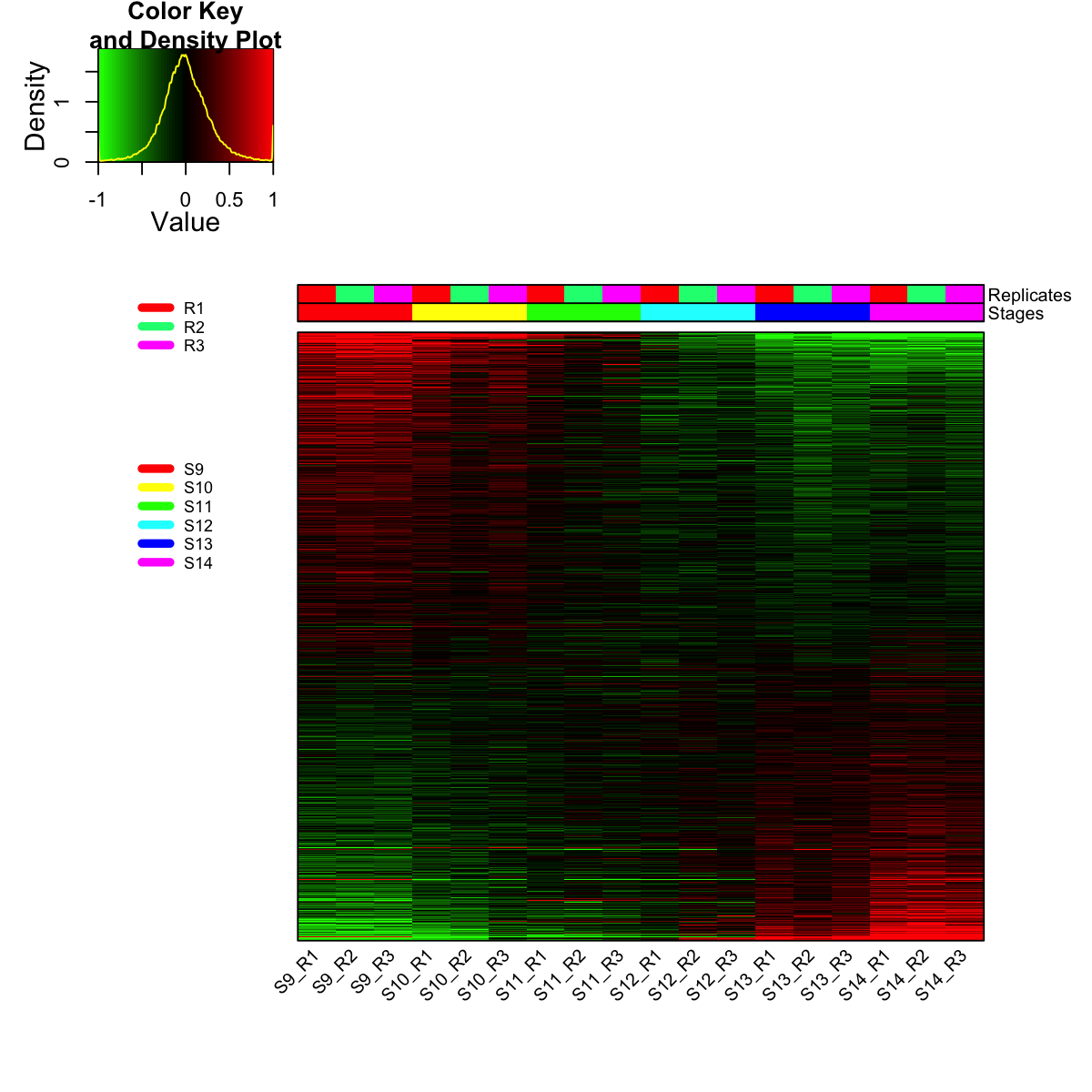
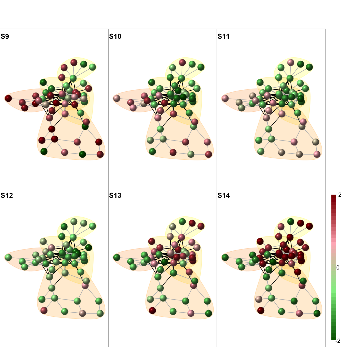
S9 S10 S11 S12 S13 S14
3125 1764 485 461 1996 2556
Start at 2015-07-21 17:43:23
First, singular value decomposition of the input matrix (with 4139 rows and 18 columns)...
Second, determinate the eigens...
via automatically deciding on the number of dominant eigens under the cutoff of 1.00e-02 pvalue
number of the eigens in consideration: 2
Third, construct the gene-specific projection vector,and calculate distance statistics...
Finally, obtain gene significance (fdr) based on 200 permutations...
doing row-wise permutations...
estimating fdr...
1 (out of 4139) at 2015-07-21 17:43:43
414 (out of 4139) at 2015-07-21 17:43:54
828 (out of 4139) at 2015-07-21 17:44:06
1242 (out of 4139) at 2015-07-21 17:44:19
1656 (out of 4139) at 2015-07-21 17:44:31
2070 (out of 4139) at 2015-07-21 17:44:43
2484 (out of 4139) at 2015-07-21 17:44:54
2898 (out of 4139) at 2015-07-21 17:45:05
3312 (out of 4139) at 2015-07-21 17:45:17
3726 (out of 4139) at 2015-07-21 17:45:29
4139 (out of 4139) at 2015-07-21 17:45:40
using stepup procedure...
Finish at 2015-07-21 17:45:40
Runtime in total is: 137 secs
Start at 2015-07-21 17:45:40
First, consider the input fdr (or p-value) distribution
Second, determine the significance threshold...
Via constraint on the size of subnetwork to be identified (30 nodes)
Scanning significance threshold at rough stage...
significance threshold: 1.00e-02, corresponding to the network size (0 nodes)
significance threshold: 1.00e-01, corresponding to the network size (441 nodes)
Scanning significance threshold at finetune stage...
significance threshold : 1.50e-02, corresponding to the network size (0 nodes)
significance threshold : 2.00e-02, corresponding to the network size (49 nodes)
significance threshold: 2.00e-02
Third, calculate the scores according to the input fdr (or p-value) and the threshold (if any)...
Amongst 4139 scores, there are 82 positives.
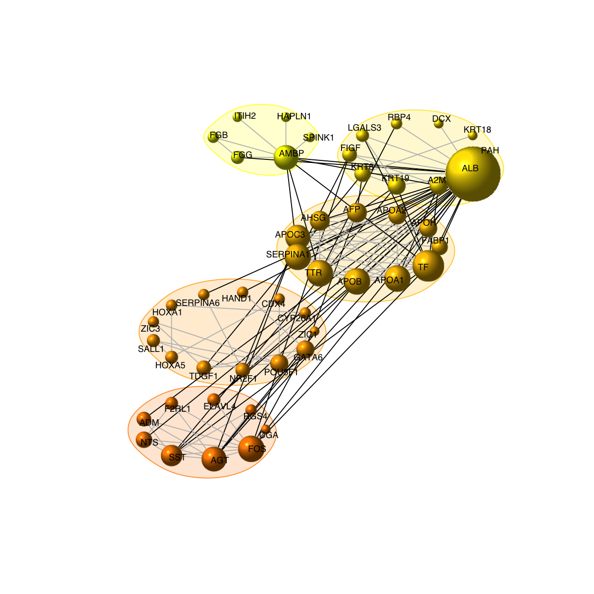
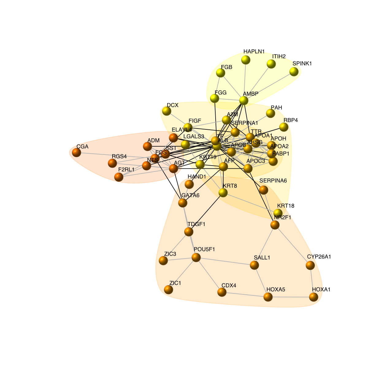
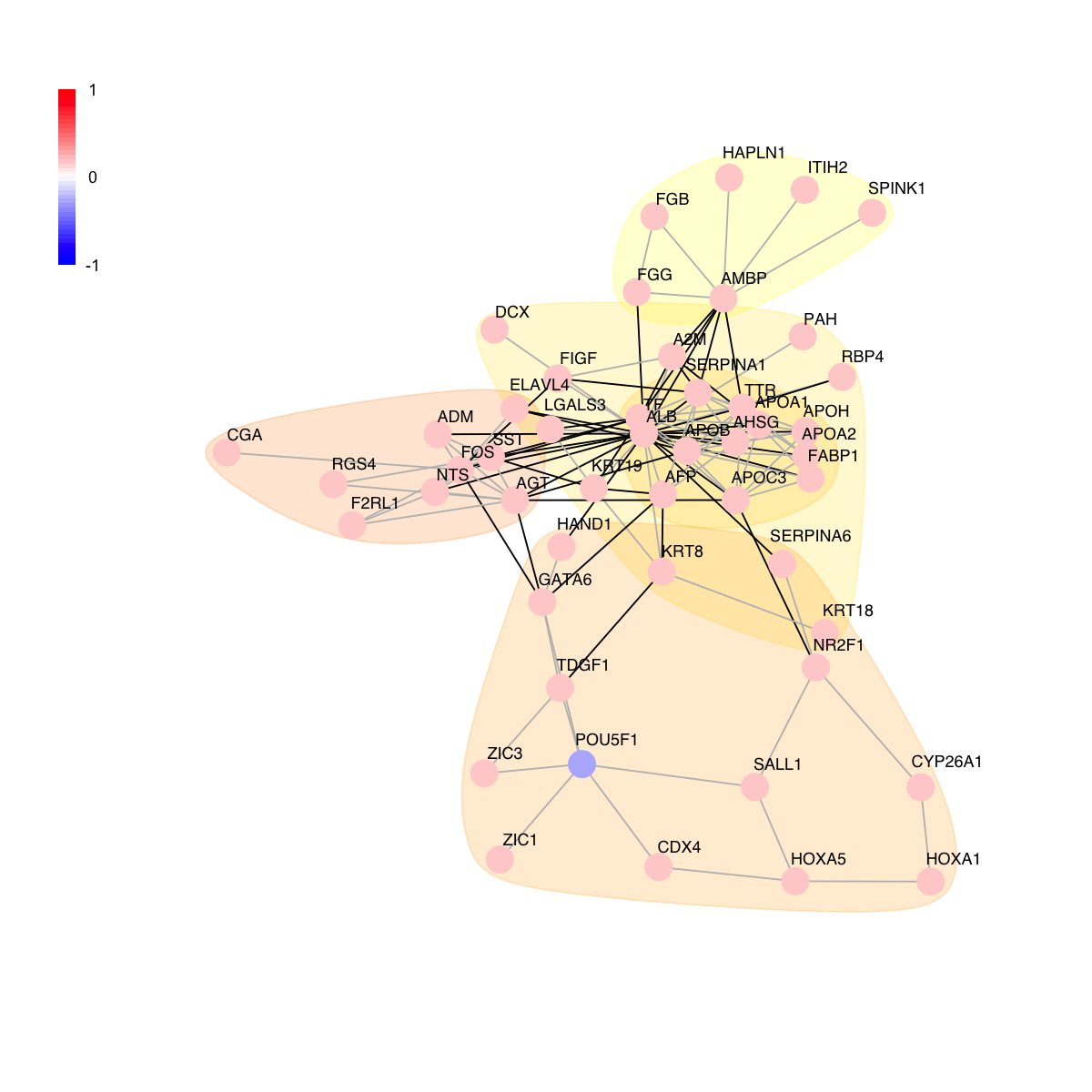
Finally, find the subgraph from the input graph with 3623 nodes and 63805 edges...
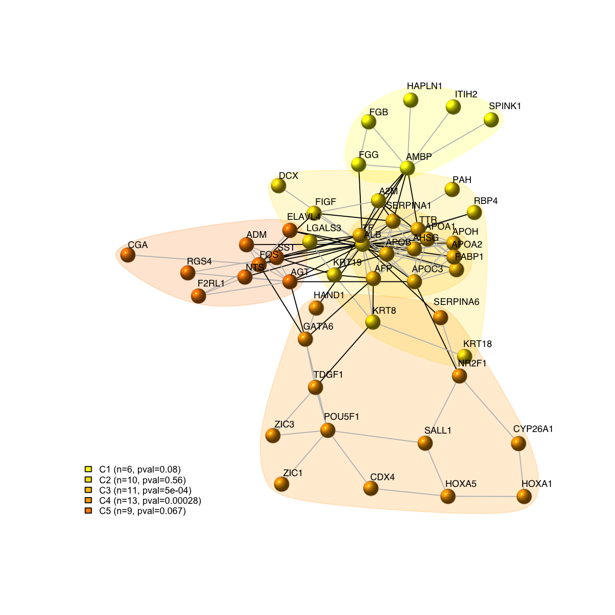
Size of the subgraph: 49 nodes and 130 edges
Finish at 2015-07-21 17:47:43
Runtime in total is: 123 secs
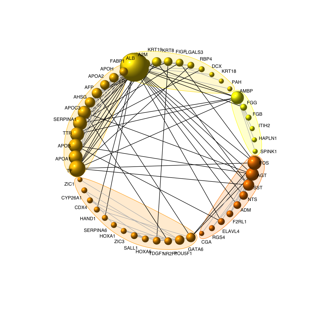
legend_name <- paste("C",1:length(mcolors)," (n=",com$csize,", pval=",signif(com$significance,digits=2),")",sep='')
legend("bottomleft", legend=legend_name, fill=mcolors, bty="n", cex=0.6)
 Start at 2015-07-21 17:48:44
First, define topology of a map grid (2015-07-21 17:48:44)...
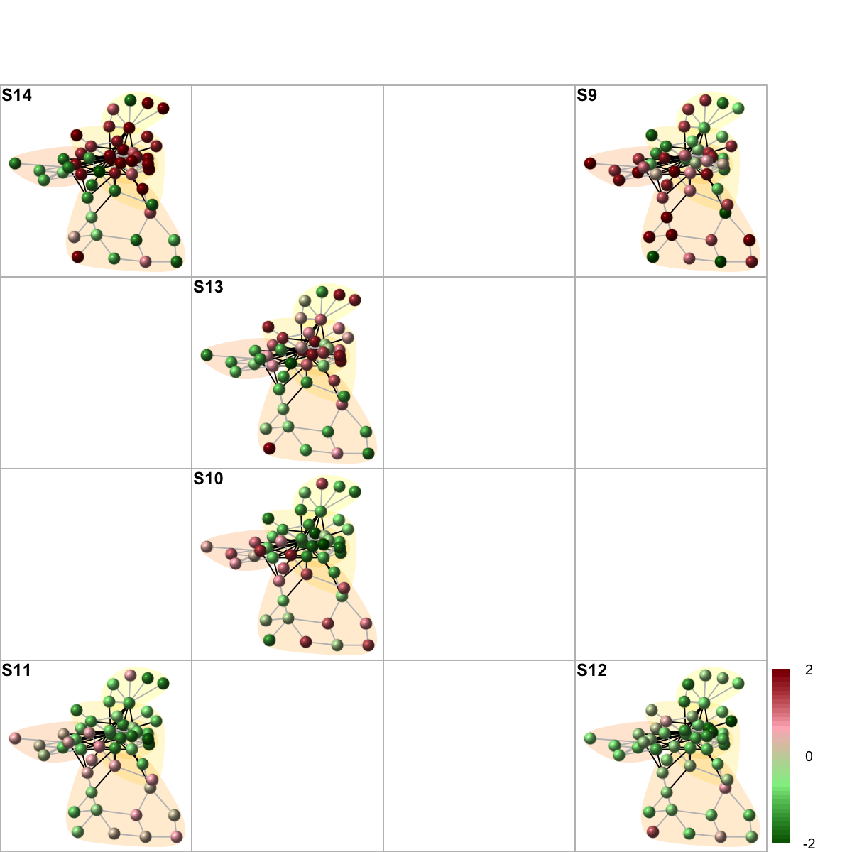
Second, initialise the codebook matrix (16 X 130) using 'linear' initialisation, given a topology and input data (2015-07-21 17:48:44)...
Third, get training at the rough stage (2015-07-21 17:48:44)...
1 out of 162 (2015-07-21 17:48:44)
17 out of 162 (2015-07-21 17:48:44)
34 out of 162 (2015-07-21 17:48:44)
51 out of 162 (2015-07-21 17:48:44)
68 out of 162 (2015-07-21 17:48:44)
85 out of 162 (2015-07-21 17:48:44)
102 out of 162 (2015-07-21 17:48:44)
119 out of 162 (2015-07-21 17:48:44)
136 out of 162 (2015-07-21 17:48:45)
153 out of 162 (2015-07-21 17:48:45)
162 out of 162 (2015-07-21 17:48:45)
Fourth, get training at the finetune stage (2015-07-21 17:48:45)...
1 out of 642 (2015-07-21 17:48:45)
65 out of 642 (2015-07-21 17:48:45)
130 out of 642 (2015-07-21 17:48:45)
195 out of 642 (2015-07-21 17:48:45)
260 out of 642 (2015-07-21 17:48:45)
325 out of 642 (2015-07-21 17:48:45)
390 out of 642 (2015-07-21 17:48:45)
455 out of 642 (2015-07-21 17:48:46)
520 out of 642 (2015-07-21 17:48:46)
585 out of 642 (2015-07-21 17:48:46)
642 out of 642 (2015-07-21 17:48:46)
Next, identify the best-matching hexagon/rectangle for the input data (2015-07-21 17:48:46)...
Finally, append the response data (hits and mqe) into the sMap object (2015-07-21 17:48:46)...
Below are the summaries of the training results:
dimension of input data: 6x130
xy-dimension of map grid: xdim=4, ydim=4
grid lattice: rect
grid shape: sheet
dimension of grid coord: 16x2
initialisation method: linear
dimension of codebook matrix: 16x130
mean quantization error: 0.429479271340322
Below are the details of trainology:
training algorithm: sequential
alpha type: invert
training neighborhood kernel: gaussian
trainlength (x input data length): 27 at rough stage; 107 at finetune stage
radius (at rough stage): from 1 to 1
radius (at finetune stage): from 1 to 1
End at 2015-07-21 17:48:46
Runtime in total is: 2 secs
Start at 2015-07-21 17:48:44
First, define topology of a map grid (2015-07-21 17:48:44)...
Second, initialise the codebook matrix (16 X 130) using 'linear' initialisation, given a topology and input data (2015-07-21 17:48:44)...
Third, get training at the rough stage (2015-07-21 17:48:44)...
1 out of 162 (2015-07-21 17:48:44)
17 out of 162 (2015-07-21 17:48:44)
34 out of 162 (2015-07-21 17:48:44)
51 out of 162 (2015-07-21 17:48:44)
68 out of 162 (2015-07-21 17:48:44)
85 out of 162 (2015-07-21 17:48:44)
102 out of 162 (2015-07-21 17:48:44)
119 out of 162 (2015-07-21 17:48:44)
136 out of 162 (2015-07-21 17:48:45)
153 out of 162 (2015-07-21 17:48:45)
162 out of 162 (2015-07-21 17:48:45)
Fourth, get training at the finetune stage (2015-07-21 17:48:45)...
1 out of 642 (2015-07-21 17:48:45)
65 out of 642 (2015-07-21 17:48:45)
130 out of 642 (2015-07-21 17:48:45)
195 out of 642 (2015-07-21 17:48:45)
260 out of 642 (2015-07-21 17:48:45)
325 out of 642 (2015-07-21 17:48:45)
390 out of 642 (2015-07-21 17:48:45)
455 out of 642 (2015-07-21 17:48:46)
520 out of 642 (2015-07-21 17:48:46)
585 out of 642 (2015-07-21 17:48:46)
642 out of 642 (2015-07-21 17:48:46)
Next, identify the best-matching hexagon/rectangle for the input data (2015-07-21 17:48:46)...
Finally, append the response data (hits and mqe) into the sMap object (2015-07-21 17:48:46)...
Below are the summaries of the training results:
dimension of input data: 6x130
xy-dimension of map grid: xdim=4, ydim=4
grid lattice: rect
grid shape: sheet
dimension of grid coord: 16x2
initialisation method: linear
dimension of codebook matrix: 16x130
mean quantization error: 0.429479271340322
Below are the details of trainology:
training algorithm: sequential
alpha type: invert
training neighborhood kernel: gaussian
trainlength (x input data length): 27 at rough stage; 107 at finetune stage
radius (at rough stage): from 1 to 1
radius (at finetune stage): from 1 to 1
End at 2015-07-21 17:48:46
Runtime in total is: 2 secs
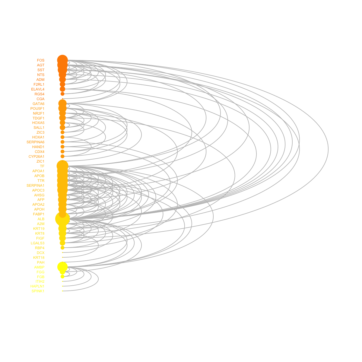
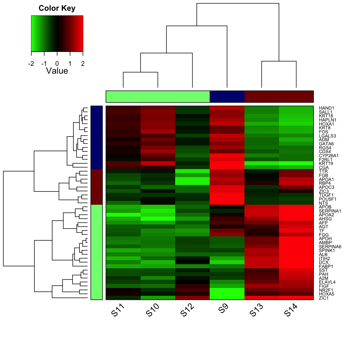
# 12) heatmap of subnetwork
visHeatmapAdv(data, colormap="gbr", row.cutree=3, column.cutree=3)
hmap <- data.frame(Symbol=rownames(data), data)
write.table(hmap, file=paste("Fang_whole.txt", sep=""), quote=F, row.names=F,col.names=T,sep="\t")
# 13) Write the subnetwork into a SIF-formatted file (Simple Interaction File)
sif <- data.frame(source=get.edgelist(g)[,1], type="interaction", target=get.edgelist(g)[,2])
write.table(sif, file=paste("Fang_whole.sif", sep=""), quote=F, row.names=F,col.names=F,sep="\t")
)
)
)
)
)
)
)
)
)
)
)
)